Modeling loans - Solutions

eCOTS 2022 - Modernizing the undergraduate regression analysis course

library(tidyverse)
library(tidymodels)
library(knitr)
library(openintro)

Introduction

The exercises below are drawn from an exam review. Students would have already completed readings, some assignments, and labs prior to attempting these questions.

You may notice some code below has already been pre-populated for you. In these cases, there is a flag set as eval = FALSE. Make sure to remove this flag prior to running the relevant code chunk to avoid any errors when rendering the document.

Data

In today’s workshop, we will explore using the tidymodels framework for modeling along with the tidyverse framework for data wrangling and visualization. We will start with some exploratory data analysis, walk through how to create the key components of a predictive model (models, recipes, and workflows), and how to perform cross-validation. Throughout we will be using the loans_full_schema dataset from the openintro package¹ and featured in the OpenIntro textbooks² .

The data has a bit of peculiarity about it, specifically the application_type variable is a factor variable with an empty level.

levels(loans_full_schema$application_type)

[1] ""           "individual" "joint"     

Let’s clean up this variable using the droplevels() function first. And let’s apply that to the whole dataset, in case there are other variables with similar issues.

loans_full_schema <- droplevels(loans_full_schema)

The variables we’ll use in this analysis are:

• interest_rate: Interest rate of the loan the applicant received.
• debt_to_income: Debt-to-income ratio.
• term: The number of months of the loan the applicant received.
• inquiries_last_12m: Inquiries into the applicant’s credit during the last 12 months.
• public_record_bankrupt: Number of bankruptcies listed in the public record for this applicant.
• application_type: The type of application: either individual or joint.

Exercises

Exercise 1: Train-test data split

Split the data into a training and test set with a 75%-25% split. Don’t forget to set a seed!

set.seed(210)

loans_split <- initial_split(loans_full_schema)
loans_train <- training(loans_split)
loans_test <- testing(loans_split)

Exercise 2: The Model

Write the model for predicting interest rate (interest_rate) from debt to income ratio (debt_to_income), the term of loan (term), the number of inquiries (credit checks) into the applicant’s credit during the last 12 months (inquiries_last_12m), whether there are any bankruptcies listed in the public record for this applicant (bankrupt), and the type of application (application_type). The model should allow for the effect of to income ratio on interest rate to vary by application type.

\[ \begin{aligned} \widehat{\texttt{interest\_rate}} = b_0 &+ b_1\times\texttt{debt\_to\_income} \\ &+ b_2 \times \texttt{term} \\ &+ b_3 \times \texttt{inquiries\_last\_12m} \\ &+ b_4 \times \texttt{bankrupt} \\ &+ b_5 \times \texttt{application\_type} \\ &+ b_6 \times \texttt{debt\_to\_income:application\_type} \end{aligned} \]

Exercise 3: EDA

Explore characteristics of the variables you’ll use for the model using the training data only.

First, take a peek at the relevant variables in the data.

loans_train %>%
  select(interest_rate, debt_to_income, term,
         inquiries_last_12m, public_record_bankrupt, application_type) %>%
  glimpse()

Rows: 7,500
Columns: 6
$ interest_rate          <dbl> 7.34, 21.85, 6.72, 17.47, 12.62, 7.34, 14.08, 1…
$ debt_to_income         <dbl> 3.81, 32.80, 4.31, 8.94, 11.87, 4.51, 20.24, 9.…
$ term                   <dbl> 36, 36, 36, 60, 60, 60, 60, 36, 60, 60, 36, 36,…
$ inquiries_last_12m     <int> 0, 1, 2, 1, 0, 1, 3, 1, 0, 0, 0, 4, 0, 0, 0, 5,…
$ public_record_bankrupt <int> 0, 0, 0, 0, 0, 0, 0, 0, 0, 0, 0, 0, 0, 0, 0, 0,…
$ application_type       <fct> individual, individual, individual, joint, indi…

Create univariate, bivariate, and multivariate plots, and make sure to think about which plots are the most appropriate and effective given the data types.

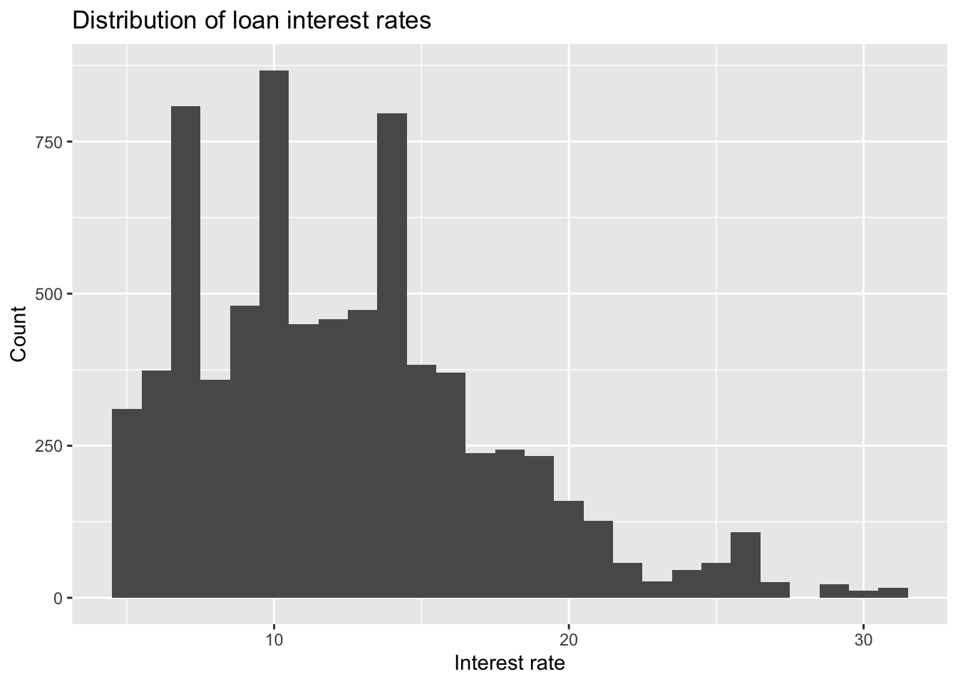
• Interest rate:

ggplot(loans_train, aes(x = interest_rate)) +
  geom_histogram(binwidth = 1) +
  labs(
    x = "Interest rate", y = "Count",
    title = "Distribution of loan interest rates"
  )

• Interest rate vs. debt to income ratio by application type:

ggplot(loans_train, 
       aes(x = debt_to_income, y = interest_rate,
           color = application_type, shape = application_type)) +
  geom_point() +
  labs(
    x = "Debt-to-income ratio", y = "Interest rate",
    color = "Application type", shape = "Application type",
    title = "Interest rate vs. Debt-to-income by application type"
  )

Warning: Removed 16 rows containing missing values (geom_point).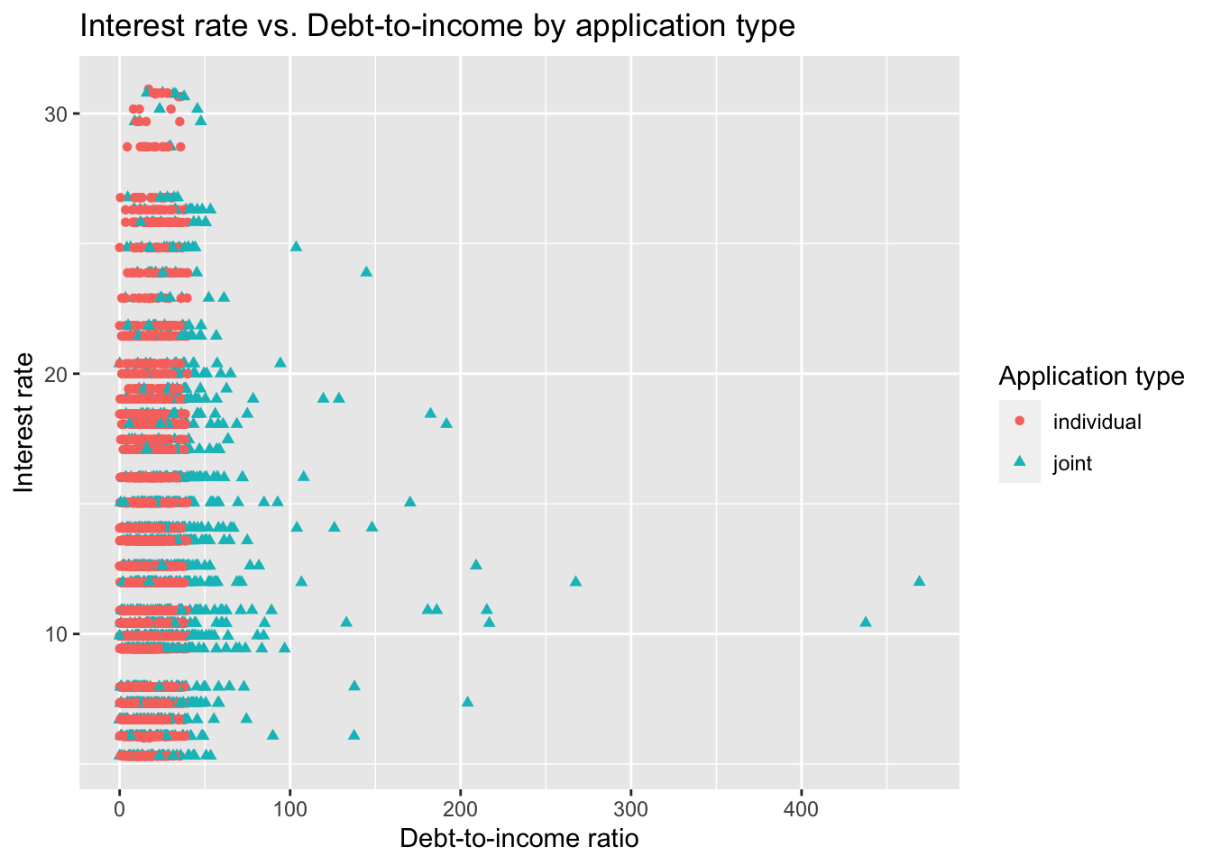

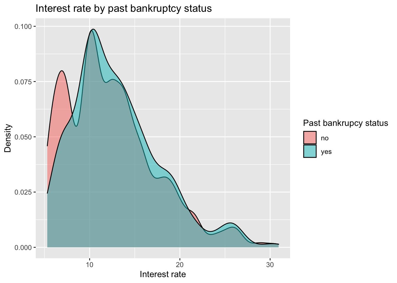
• Interest rate by bankruptcy:

loans_train %>%
  mutate(bankrupt = if_else(public_record_bankrupt == 0, "no", "yes")) %>%
  ggplot(aes(x = interest_rate, fill = bankrupt)) +
  geom_density(alpha = 0.5) +
  labs(
    x = "Interest rate", y = "Density",
    fill = "Past bankrupcy status", 
    title = "Interest rate by past bankruptcy status"
  )

Exercise 4: Model specification

Specify a linear regression model. Call it loans_spec.

loans_spec <- linear_reg()

Exercise 5: Recipe and formula building

• Predict interest_rate from debt_to_income, term, inquiries_last_12m, public_record_bankrupt, and application_type.
• Mean center debt_to_income.
• Make term a factor.
• Create a new variable: bankrupt that takes on the value “no” if public_record_bankrupt is 0 and the value “yes” if public_record_bankrupt is 1 or higher. Then, remove public_record_bankrupt.
• Interact application_type with debt_to_income.
• Create dummy variables where needed and drop any zero variance variables.

loans_rec <- recipe(interest_rate ~ debt_to_income +
  term + inquiries_last_12m +
  public_record_bankrupt + application_type,
data = loans_train
) %>%
  step_center(debt_to_income) %>%
  step_mutate(term = as_factor(term)) %>%
  step_mutate(bankrupt = as_factor(if_else(public_record_bankrupt == 0, "no", "yes"))) %>%
  step_rm(public_record_bankrupt) %>%
  step_dummy(all_nominal_predictors()) %>%
  step_interact(terms = ~ starts_with("application_type"):debt_to_income) %>%
  step_zv(all_predictors())

Exercise 6: Creating a workflow

Create the workflow that brings together the model specification and recipe.

loans_wflow <- workflow() %>%
  add_model(loans_spec) %>%
  add_recipe(loans_rec)

Exercise 7: Cross-validation and summary

Conduct 10-fold cross validation.

set.seed(210)
loans_folds <- vfold_cv(loans_train, v = 10)
loans_fit_rs <- loans_wflow %>%
  fit_resamples(loans_folds)
loans_fit_rs

# Resampling results
# 10-fold cross-validation 
# A tibble: 10 × 4
   splits             id     .metrics         .notes          
   <list>             <chr>  <list>           <list>          
 1 <split [6750/750]> Fold01 <tibble [2 × 4]> <tibble [0 × 3]>
 2 <split [6750/750]> Fold02 <tibble [2 × 4]> <tibble [0 × 3]>
 3 <split [6750/750]> Fold03 <tibble [2 × 4]> <tibble [0 × 3]>
 4 <split [6750/750]> Fold04 <tibble [2 × 4]> <tibble [0 × 3]>
 5 <split [6750/750]> Fold05 <tibble [2 × 4]> <tibble [0 × 3]>
 6 <split [6750/750]> Fold06 <tibble [2 × 4]> <tibble [0 × 3]>
 7 <split [6750/750]> Fold07 <tibble [2 × 4]> <tibble [0 × 3]>
 8 <split [6750/750]> Fold08 <tibble [2 × 4]> <tibble [0 × 3]>
 9 <split [6750/750]> Fold09 <tibble [2 × 4]> <tibble [0 × 3]>
10 <split [6750/750]> Fold10 <tibble [2 × 4]> <tibble [0 × 3]>

Summarize metrics from your CV resamples.

collect_metrics(loans_fit_rs)

# A tibble: 2 × 6
  .metric .estimator  mean     n std_err .config             
  <chr>   <chr>      <dbl> <int>   <dbl> <chr>               
1 rmse    standard   4.54     10 0.0363  Preprocessor1_Model1
2 rsq     standard   0.173    10 0.00646 Preprocessor1_Model1

We can also visualize the metrics across folds.

collect_metrics(loans_fit_rs, summarize = FALSE) %>%
  mutate(id = str_remove(id, "Fold")) %>%
  ggplot(aes(x = id, y = .estimate, group = .metric)) +
  geom_line() +
  facet_wrap(~.metric, scales = "free", ncol = 1) +
  labs(x = "Fold", y = "Estimate",
       title = "Cross-validation metrics")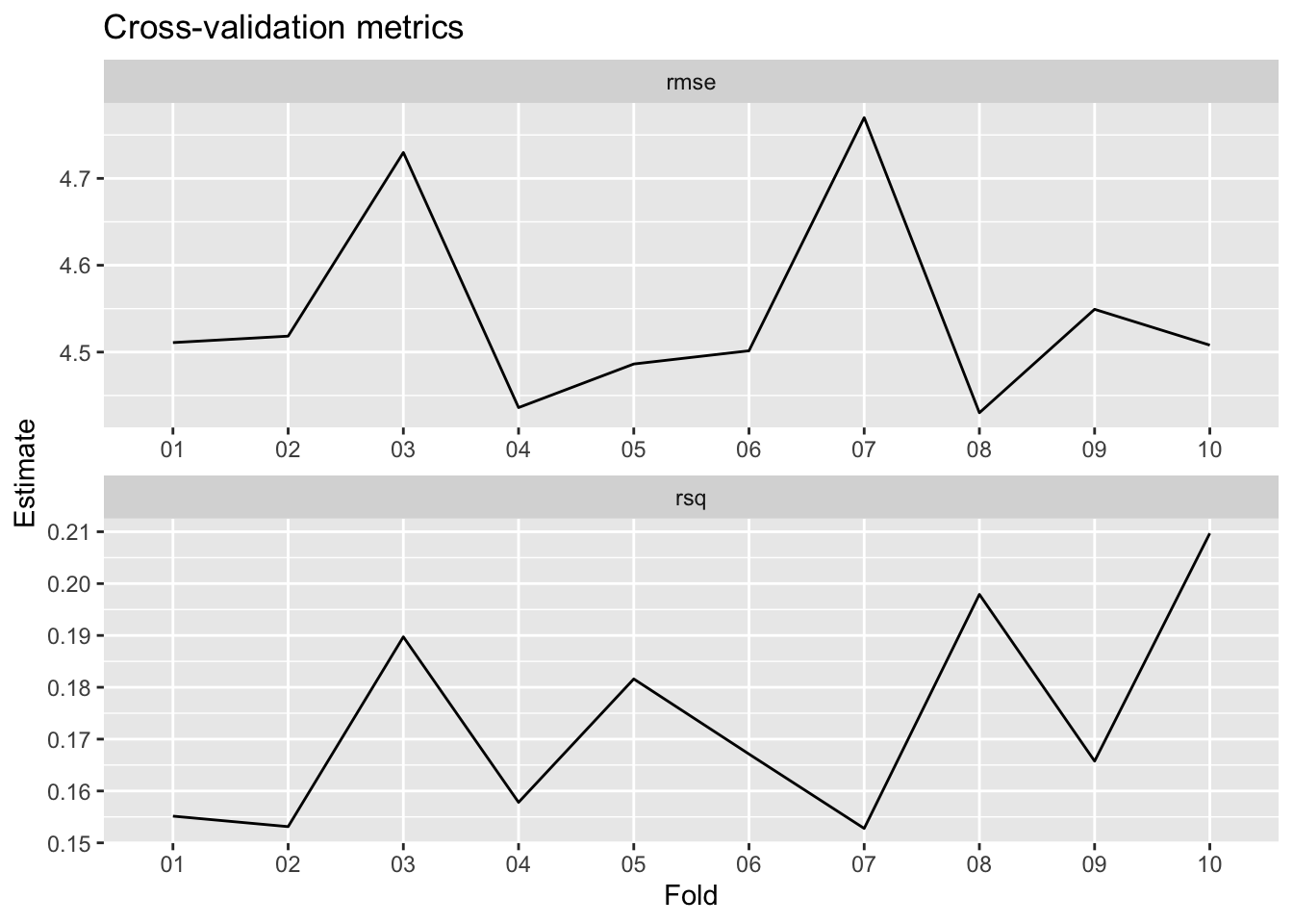

Writing Exercise

In this exercise, we will synthesize our work above to create a reader-friendly version of our conclusions. In the classroom, these sorts of writing exercises appear throughout homework and lab assignments as well as exams. They give students an opportunity to demonstrate their understanding while gaining an appreciation that communication is a crucial part of using statistics.

Exploratory data analysis

Using your plots above (along with any other metrics you compute), describe your initial findings about the training data. Discuss why we perform EDA only on the training data and not on the entire data set.

loans_med <- median(loans_train$interest_rate)
loans_iqr <- IQR(loans_train$interest_rate)

It appears that the marginal distribution for interest rates is largely unimodal (possibly bimodal since there aren’t many loans issued with interest rates around 7%) with a right-skew. The median interest rate is 11.98 with IQR 5.62.

It appears that there is no strong relationship between debt-to-income when the debt-to-income ratio is low. It seems that the that joint applications generally have higher debt-to-income ratios, but possibly some lower interest rates for highly levered (i.e., high debt-to-income ratios, especially greater than 100%) applications. These may be outliers.

The boxplot seems to suggest that while applications with a bankruptcy history have higher interest rates, the difference is very slight.

Model fitting and fit evaluation

Although our primary aim is prediction and not inference, it may be of interest to view the model fit nonetheless to make sure nothing looks out of the ordinary. Create a neatly organized table of the model output, and describe your observations, such as which parameters are significant. Make sure to interpret some coefficients appropriately.

loans_train_fit <- fit(loans_wflow, data = loans_train)

tidy(loans_train_fit) %>% 
  kable(digits = 2)

term	estimate	std.error	statistic	p.value
(Intercept)	10.94	0.08	135.05	0.00
debt_to_income	0.11	0.01	16.46	0.00
inquiries_last_12m	0.22	0.02	9.91	0.00
term_X60	3.84	0.11	33.41	0.00
application_type_joint	-0.08	0.16	-0.53	0.59
bankrupt_yes	0.46	0.16	2.84	0.00
application_type_joint_x_debt_to_income	-0.09	0.01	-12.00	0.00

From the above table, it appears that all of the coefficients are significant at the 0.05 significance level except for application_type. However, the interaction with debt_to_income is significant, so we want to include the main effect. We find that the sign of the coefficients is intuitive. For instance, as the debt-to-income ratio increases by 1%, the interest rate is predicted to increase by about 0.11% on average, holding all equal. Similarly, relative to loans with a 3-year maturity, loans with a 5-year maturity are predicted to have an interest rate about 3.84% higher on averaged, all else equal.

Cross-validation

Explain what 10-fold CV does, and why it’s useful. Display a neat table with the outputs of your CV summary, and describe your observations. Make sure to discuss why we are focusing on R-squared and RMSE instead of adjusted R-squared, AIC, and BIC.

10-fold CV splits the training data into roughly 10 equal groups, fits the model on 9 of the groups, and then tests the performance on the remaining 10th group. This is done by leaving one group out at a team, and then averaging the error. We do this because even though we cannot use the test data to in fitting the model, this allows us to get an idea of how well our model performs on data it has not seen before. In turn, we can compare different models based on their predictive performance using metrics like R-squared and RMSE. Since prediction is our primary concern, we use these metrics instead of R-squared, AIC, and BIC.

cv_metrics <- collect_metrics(loans_fit_rs)
cv_metrics %>% kable(digits = 2)

.metric	.estimator	mean	n	std_err	.config
rmse	standard	4.54	10	0.04	Preprocessor1_Model1
rsq	standard	0.17	10	0.01	Preprocessor1_Model1

loan_rmse <- cv_metrics$mean[1]
loan_rsq <- cv_metrics$mean[2]

The above table computes the RMSE, which is about 4.54, and the R-squared, which is about 0.17.

Footnotes

1. Mine Çetinkaya-Rundel, David Diez, Andrew Bray, Albert Y. Kim, Ben Baumer, Chester Ismay, Nick Paterno and Christopher Barr (2022). openintro: Data Sets and Supplemental Functions from ‘OpenIntro’ Textbooks and Labs. R package version 2.3.0. https://CRAN.R-project.org/package=openintro.

2. Mine Çetinkaya-Rundel and Johanna Hardin. 2021. OpenIntro::Introduction to Modern Statistics. https://openintro-ims.netlify.app.